U.S. Economic Growth Update

Is the Hormuz Shock a Productivity Regime Shifter?

The last issue of this series went deep into the weeds on the impact of a de-immigration induced demographic sudden stop on growth and inflation. The conclusions were:

• The labor market would tighten (lower U3) without triggering a wage-driven inflationary impulse due to the ongoing productivity boom and the remaining slack in the under-30 age cohort of the labor market.

• The Administration’s immigration policies would reduce aggregate consumer spending and lower GDP output between 75-basis points and 1%, further putting a lid on labor market-driven wage pressures.

• The gargantuan AI spend cycle would be net supportive and additive to growth, resulting in a goldilocks environment of less inflation by year-end and a continuation of the growth cycle.

A few days ago, it was observed that the K-shaped nature of aggregate labor income distribution and the nature of higher oil prices acting as a regressive consumption tax that lowers discretionary spending, would dampen any inflationary impulse from temporary higher oil prices.

Today, increasing spot inflation mixed with lower aggregate demand brings back 2022 vibes.

Recall the defining macroeconomic events of 2022:

• The largest oil supply shock since the 1970’s, resulting in the largest price shock since the late 1980’s.

• In response to being late to the inflationary trade, the Powell Fed embarked on its most aggressive hiking cycle since Volker and yield curve maxxed until inversion.

• Two back-to-back quarters of negative GDP growth in 2022 (one revised upward, one still negative) but no technical NBER recession that everyone was sure would come.

• A kinetic geopolitical event between Russia and Ukraine.

• For the full year 2022, the U.S. economy expanded by 2.1%. This growth was primarily driven by consumer spending, exports, and private inventory investment, which helped offset a decrease in residential fixed investment and federal government spending.

• A white-hot labor market that saw the U3 unemployment rate fall from 4.0% to 3.5%, and average 3.64% for the year was foundational to the above.

One quarter into 2026, and the U.S. economy is now faced with another set of supply and price shocks, and a labor market that while shrinking and mechanically lowering U3, still hasn’t produced any net new jobs in over a year.

Is it so over? Let’s Dive in.

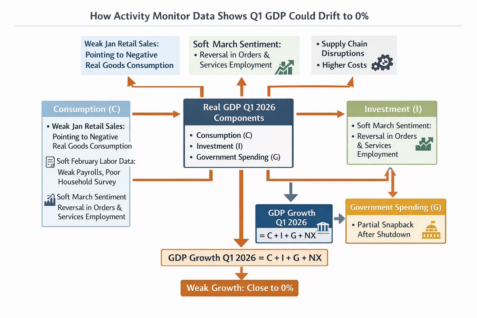
The Strait of Hormuz shock adds a new layer of risk to the economic backdrop for H1 2026. If supply chain disruptions materially constrain energy, chemical, and other manufacturing inputs as they did in 2022, two back-to-back quarters of negative GDP go from a left tail risk to a base case.

• Recall, 2026 Q1 GDP started on the soft side due to the lagged effects of the government shutdown and subsequent layoffs in Q4 2025.

• Prior to the Hormuz shock, soft data was pointing towards a mid-quarter cyclical acceleration.

The current shock will most likely drift Q1 GDP closer to zero but likely keep it positive because of the mid-quarter momentum.

• Higher commodity prices will directly and indirectly depress consumer spending (demand destruction).

• A resumption of government spending post-shutdown offers a modest offset.

• Even if unemployment doesn’t spike sharply, sluggish employment growth still reduces spending growth in the context of a price shock, which shows up as softer PCE (consumer expenditures, not the price index) when the BEA compiles quarterly GDP.

On the production side, business investment, production and inventories will be impacted.

• Disruptions in supply chains (e.g., due to energy/price shocks), force firms to produce less, and order fewer inputs.

• Business investment is also negatively impacted and contributes negatively to GDP as part of the investment component.

• If inventories shrink because firms sell stored goods without replacement, that also subtracts from GDP.

Mechanically, GDP growth = C + I + G + (X−M)

Q2 will simply be a larger, more leveraged version of this.

A baseline of 1-month of kinetic conflict takes the shock and disruptions into April. In a perfect world, it will still take months before capacity and activity come back online at the oil and refinery level, much less actual deliveries and distribution to end-producers.

Thus, the biggest issue after kinetic conflict ends is the normalization and sequencing road ahead.

The global supply chain faces a non-compressible, sequential recovery timeline. It is a biological restart for an industrial system, not a light switch.

• Port bottlenecks and backlogs will take approximately one week to work off, as an oil tanker needs to visit 2-3 ports to top-off 2 million in barrel capacity.

• Once the initial buffer of stored oil is shipped out, oilfields need to come back online. This process can take two weeks to revive pumping systems, pressure, and systems safety. Of course, this assumes there are no damages from military strikes, or shortages of spare replacement parts. Bruh. 👀

• After oilfields come back online, refineries need to come to life. This is not just an engineering and production effort. Refineries don’t fire up for a single tanker; they need visible tanker flow that results from a negotiated political settlement between the military antagonists. Another two weeks. ✅

• After basic refining (the first phase of distillation), oil products need to go to a steam cracker for additional processing to turn them into things like gasoline. Steam crackers need to wait for the refineries to be operational. Without a refined product as an input, there is nothing to “crack”. This can take four to six weeks.

In a normal to perfect scenario, the world is looking at eleven to twelve weeks petrol supply chain normalization after the cessation of hostilities. If repairs are required, or hostilities resume, the timeline shifts out.

Thus, Pinebrook is writing off Q2 GDP as a zero, and potentially negative.

The inflection from a mini-cyclical pop to recession-like GDP is not the main event; it misses the forest for the trees. GDP can be volatile in the short term and be fine in the longer term.

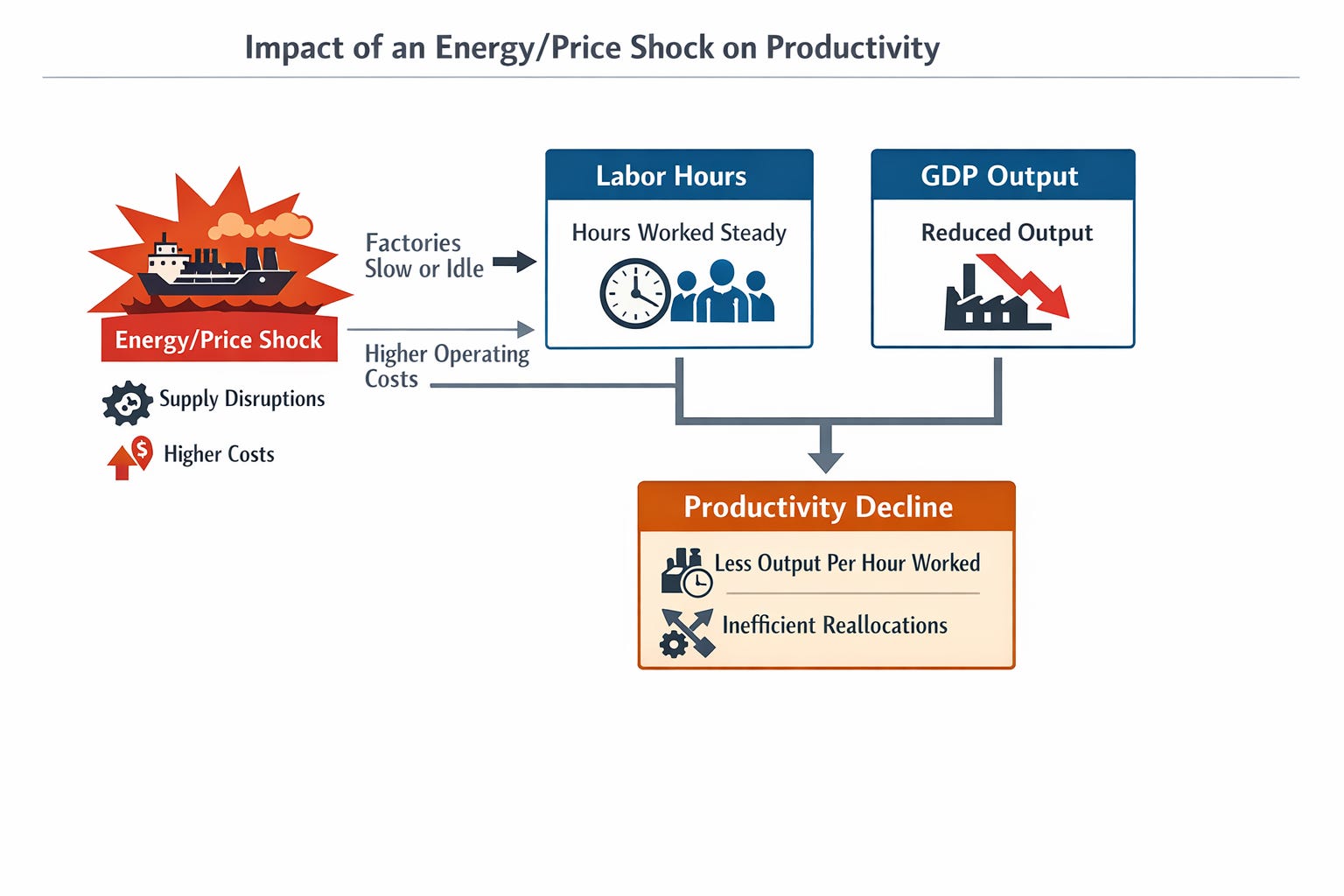
Productivity is going to take a hit.

• A GDP slowdown doesn’t automatically equal lower productivity - but in this context, it does.

• Productivity is generally measured as output per hour worked (or output per worker).

• A GDP slowdown can affect productivity in different ways depending on why output is falling and how labor hours respond.

• If output falls but hours worked fall proportionally, measured productivity may not change much.

• If output falls but hours worked do not fall proportionally, productivity declines because workers are producing less per hour.

In the case of an energy/price shock, the second scenario above is the likely result.

• A disruption in key manufacturing inputs (chemicals, metals, etc.) reduces available output as some factories cannot operate at full capacity due to missing inputs or high energy costs.

• Production becomes intermittent or staggered to conserve energy or inputs.

• Economies of scale go down, and marginal costs go up, which impacts productivity and shows up in profit margins.

Second order effects result from reallocations and inefficiencies.

• Firms may shift production or inputs in response to price shocks, which can be disruptive and reduce efficiency.

• Workers may be reassigned, idled, or underutilized while supply chain gaps persist.

• Higher energy prices can raise the cost of capital-intensive production, slowing investment in productivity-enhancing projects.

Public spending might maintain aggregate demand and keep the labor market from falling apart, but won’t make private manufacturing or services more efficient.

Recall, supply chain abundance is one of the three pillars (along with a mature labor market and a fixed investment boom) that underwrites the pro-cyclical productivity boom that was front run and called on these pages in 2024.

These three pillars led to lower inflation and anchored expectations and allowed fixed non-residential investment (hello, Ai CapEx) to expand without policy tightening.

• The above is best characterized as an abundance regime, and it was the first time since the late 90’s that the U.S. economy was in an abundance regime.

• Prior productivity booms were countercyclical, typically coming out of a recession after an employment extinction event, where productivity mechanically went up as firms did more with less people.

• The 2025 tariff trade policies strained supply chain abundance by raising prices and distorting supply lines, causing shifts and new bottlenecks.

• An energy supply shock adds further pressure to supply chain abundance, at a scale that ripples through the entire economic system.

The macroeconomic risk of 2026 is not a pullback in GDP or a one-off price shock. It is the growing risks to the post-pandemic abundance regime.

What happens when supply abundance disappears?

Instead of:

Demand ↑ → Investment ↑ → Productivity ↑

You get:

Demand ↑ → Input costs ↑ → Output constrained

Then three things happen.

• Production becomes constrained. Energy shocks, commodity shortages, or logistics disruptions mean factories are idle, production schedules break, and inventories fall. Workers can remain employed, but they produce less output per hour.

• Investment then becomes defensive. Instead of investing in capacity and efficiency, firms invest in resiliency. Inventory buffers, redundant suppliers, domestic reshoring, energy hedging. These are resilience investments, not efficiency investments.

• Inflation crowds out demand if energy/food/housing prices spike. Households must allocate more income to essentials. If essentials become expensive, then discretionary demand falls, investment falls, and productivity slows.

Without supply chain abundance, procyclical productivity shifts from optimization to constraint management; from efficiency maxxing to surviving supply shortages and their associated costs.

A supply shock doesn’t immediately kill pro-cyclical productivity. But over time, it can break the regime. There are two possible paths from here.

Temporary shock.

• Productivity dips.

• Supply chains normalize.

• Productivity resumes.

This is what happened after the pandemic.

Persistent supply instability.

• Investment shifts toward resilience.

• Costs rise structurally.

• Productivity regime ends.

That’s essentially what happened after 1973.

If the 2026 Hormuz supply chain disruption kills the abundance regime, the macro regime shifts down from its current 1990’s-style growth.

However, a 1970’s-style supply constrained economics is not the base case.

To get a 1970’s-style constraint economic regime requires the elements discussed in a recent note:

• A wage-price spiral emanating from union negotiated labor contracts.

• A non-credible monetary authority.

• A higher energy intensity for the economy than what we have now – effectively walking back the structure of the economy by 40-years.

In addition to the above, the service sector would need to shrink, and U.S. energy production would need to deteriorate.

What could happen, is a hybrid regime characterized by moderate inflation + weak productivity + volatile growth. Think less 70’s stagflation and more early 2010’s with an inflationary twist.

The natural question is, how long do we have before the supply shock starts to transition the economy into a regime discussed above?

The short answer is, it doesn’t take very long if the shock is persistent. The transition from a supply-abundance regime to a low productivity supply constrained economy historically happens over roughly 4–8 quarters, not decades.

The key is whether the shock is temporary price volatility or persistent supply instability.

Let’s walk through the mechanics.

• A supply shock must persist long enough to change firm behavior. Firms initially treat shocks as temporary. But once they conclude the shock is structural, they start changing supply chains, investment strategy, inventory policy, and pricing behavior.

• That behavioral shift is what creates a regime change. Historically, firms begin making those structural adjustments after about 12–18 months of instability.

The timeline of a regime shift.

Phase 1 — Immediate shock (0–3 months).

• Energy or supply disruption hits.

• Commodity prices spike.

• Production disruptions appear.

• Inventories begin falling.

• GDP growth slows.

Productivity usually does not collapse yet because firms still expect normalization. This is where we currently are in the early stage of a shock.

Phase 2 - Adjustment period (3–9 months)

Firms start realizing the shock may persist. You begin to see:

• Inventory hoarding.

• Supplier diversification.

• Longer delivery times.

• Defensive capex.

Productivity begins weakening because firms prioritize resilience over efficiency. GDP growth becomes volatile.

Phase 3 — Structural shift (9–24 months)

If supply instability continues, the economy transitions to a constrained regime.

• Structurally higher commodity prices.

• Lower productivity growth.

• Higher inflation volatility.

• Weaker investment efficiency.

This is when the economy starts losing abundance, and while it may not resemble that 70’s show, it does begin to look more…..European.🇪🇺

Now, historically, productivity slowdowns do not appear evenly across the economy. They propagate in a fairly consistent order because some sectors sit closer to physical supply chains and energy inputs than others.

Sectoral sequencing is one of the clearest early-warning signals that a supply-constraint regime is emerging. Below is the typical sequence seen during major supply shocks (1970s oil shocks, 2007–08 commodity shock, and to some extent the 2021 supply-chain crisis).

Transportation & Logistics (first sector to break)

This sector is usually the first sector productivity deteriorates because fuel is a dominant cost input. Shipping routes are sensitive to disruptions, and supply chain congestion creates idle labor and equipment.

When energy prices spike or shipping routes are disrupted, logistics companies often have

trucks waiting for loads, ships waiting in ports, and warehouses waiting for inputs. Workers remain employed, but throughput falls, so output per hour declines.

Typical signals

• Rising freight rates.

• Longer delivery times.

• Declining transport productivity.

• Historically this shows up 3–6 months after a supply shock begins.

Manufacturing (second stage)

Manufacturing is usually the second sector affected because it relies heavily on upstream inputs (chemicals, metals, energy) and production lines depend on synchronized supply chains. When inputs become scarce, production lines stop intermittently, workers wait for materials, and plants run below capacity. This creates a sharp drop in manufacturing output per worker.

Typical signals

• Falling capacity utilization.

• Rising inventories of unfinished goods.

• Declining manufacturing productivity.

• Historically this stage appears 6–12 months after the initial shock.

Construction (third stage)

Construction is extremely sensitive to energy costs and materials (steel, cement, lumber) and financing conditions. When commodity prices rise, projects are delayed, budgets are revised, labor is underutilized. Construction productivity therefore weakens as projects stretch out over longer timelines.

Typical signals

• Slower housing starts.

• Project delays.

• Rising building costs.

• This stage often occurs 9–15 months after the shock.

Consumer goods

After the upstream sectors weaken, the effects begin to hit consumer-facing industries. Retail and consumer goods firms experience rising inventory costs, weaker discretionary demand, and pressure to cut operating costs. Productivity falls because firms maintain staffing levels while sales growth slows.

This stage tends to appear 12–18 months into the cycle.

Services (last sector affected).

Services usually experience the slowest productivity adjustment because they are less dependent on physical supply chains. However, they are eventually affected through higher energy costs, slower consumer spending, and rising wage costs.

Why this sequence matters.

Because productivity is measured across the whole economy, early deterioration in logistics or manufacturing does not immediately show up in aggregate productivity statistics. Instead, it gradually spreads across sectors.

By the time aggregate productivity weakens significantly, the supply shock has usually been present for multiple quarters.

When logistics and manufacturing productivity weaken simultaneously, it often signals that the economy is moving from efficiency optimization toward constraint management.

Why Any of This Matters

Productivity determines how efficiently firms convert labor and capital and other resources into output.

• When productivity rises, unit costs fall and margins expand, supporting higher corporate earnings and equity valuations.

• When productivity weakens - particularly due to supply disruptions - costs per unit rise, margins come under pressure, and investors may reassess expected profitability, leading to lower valuations or multiple compression.

• High-productivity environments typically support higher multiples because margins are stable or rising.

• When productivity weakens, margins become more volatile, cost pressures increase, growth becomes less efficient, and investors demand a lower valuation multiple to compensate for increased risk.

• Periods of strong productivity growth - such as the late 1990s and the post pandemic era - are associated with rising corporate margins, high returns on capital, and expanding equity valuation multiples.

• Conversely, during supply-driven cost shocks (e.g., energy spikes or supply chain disruptions), margins often narrow and valuations reset lower.

Concluding Remarks

• Near zero GDP growth is a baseline expectation for Q1 2026, and potential negative for Q2 2026.

• Even an early end to hostilities kicks the timeline for supplies coming back online to Q3 2026.

• General price normalization (in core PCE terms, not oil) would follow over the following year, if not longer.

• If the supply shock persists for over 4-8 quarters, the supply abundance regime is at risk and comes into question.

• Should the above happen, the U.S. economy would likely not resemble that of the 1970s, but become more European in its productivity and growth outlook.

• A sectoral sequencing has been laid out to describe the evolution of the above.

• A structural productivity shift caused by an end to the abundance regime would lower corporate earnings, valuations and introduce volatility into financial markets.

• Navigating structural shifts in the economy will be a north star to managing risk in financial markets in 2026.